Stanford CS336 | Language Modeling from Scratch | 02

前言

课程链接：Language Modeling from Scratch

第二课是 Pytorch，Resource Accounting

Overview of this lecture:

• We will discuss all the primitives needed to train a model.
• We will go bottom-up from tensors to models to optimizers to the training loop.
• We will pay close attention to efficiency (use of resources).

pay close attention to 关注；抓紧

In particular, we will account for two types of resources:

• Memory (GB)
• Compute (FLOPs)

napkin math

# Question: 
# How long would it take to train a 70B parameter model on 15T tokens on 1024 H100s?

total_flops = 6 * 70e9 * 15e12  # @inspect total_flops

assert h100_flop_per_sec == 1979e12 / 2

mfu = 0.5

flops_per_day = h100_flop_per_sec * mfu * 1024 * 60 * 60 * 24  # @inspect flops_per_day

days = total_flops / flops_per_day  # @inspect days

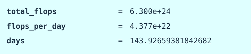
total_flops这个公式来源于一个经典经验公式：

训练一个 Transformer 模型，大约需要 6 × 模型参数数量 × token 数量 的浮点运算（FLOPs）

为什么是 6？

这个是经验值，参考自 OpenAI 的 GPT 和 Google 的 PaLM 等论文，它考虑了：

• 前向传播
• 反向传播
• 梯度更新
• 优化器状态维护（比如 Adam）
• 冗余操作（比如 dropout、layer norm）

跳回（刚看不用点）

h100_flop_per_sec

H100 FP8 理论最大吞吐量为约 1979 TFLOPs（每秒 $1.979×10^{15}$）

但是，这里除以 2 是为了得到更现实的 FP16/BF16 性能。在实际训练中我们通常使用混合精度（BF16/FP16）

MFU(Model Flop Utilization)

MFU（Model Flop Utilization）是一个效率指标，代表：

实际模型训练时使用的 FLOPs / 理论可用的 FLOPs

理想情况下 MFU = 1（完美利用），但实际中受限于：

• 通信延迟（特别是大模型并行）
• 内存带宽瓶颈
• 计算空闲

# Question: 
# What's the largest model that can you can train on 8 H100s using AdamW (naively)?
h100_bytes = 80e9  # 每张 H100 有 80 GB = 80 × 10⁹ 字节
bytes_per_parameter = 4 + 4 + (4 + 4)  # parameters, gradients, optimizer state  
num_parameters = (h100_bytes * 8) / bytes_per_parameter
# Caveat 1: we are naively using float32 for parameters and gradients. 
# We could also use bf16 for parameters and gradients (2 + 2) and keep an extra float32 copy of the parameters (4). This doesn't save memory, but is faster.  [Rajbhandari+ 2019]
# parameters, gradients 用 bf16（2 + 2 字节），再保存一份 float32 copy（4 字节），内存不省但计算更快。
# Caveat 2: activations are not accounted for (depends on batch size and sequence length).
# 激活值的内存占用跟 batch size、序列长度和层数强相关，但这里没考虑。

bytes_per_parameter

项目	意义	所占字节（float32）
4	参数本身（weights）	4 字节
4	梯度（gradients）	4 字节
4	AdamW 的一阶动量（m）	4 字节
4	AdamW 的二阶动量（v）	4 字节
合计	每个参数所需内存总量	16 字节

这是 float32 情况下常见的“训练态显存需求”估算。

如果用 float32 精度 和 AdamW 优化器，在 8 张 H100（共 640 GB 显存） 上最多能训练一个 40B 参数规模的模型。

Tensor

介绍了一下tensor的基本用法：

x = torch.tensor([[1., 2, 3], [4, 5, 6]])  # @inspect x
x = torch.zeros(4, 8)  # 4x8 matrix of all zeros @inspect x
x = torch.ones(4, 8)  # 4x8 matrix of all ones @inspect x
x = torch.randn(4, 8)  # 4x8 matrix of iid Normal(0, 1) samples @inspect x
x = torch.empty(4, 8)  # 4x8 matrix of uninitialized values @inspect x
nn.init.trunc_normal_(x, mean=0, std=1, a=-2, b=2)  # @inspect x

float32

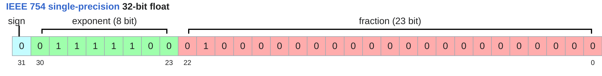
单精度浮点数，他还开玩笑说在科学计算中不是双精度我不认的~

深度学习可以随意一点

x = torch.zeros(4, 8)  # @inspect x
assert x.dtype == torch.float32  # Default type
assert x.numel() == 4 * 8
assert x.element_size() == 4  # Float is 4 bytes
assert get_memory_usage(x) == 4 * 8 * 4  # 128 bytes

float16

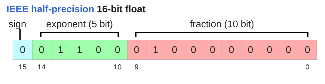
半精度浮点数

这里主要是说fp16的精度问题

x = torch.tensor([1e-8], dtype=torch.float16)  # @inspect x
assert x == 0  # Underflow!

浮点数计算问题： 计算0.01的二进制表示

步骤	乘法	整数部分	小数部分
1	0.01 × 2 = 0.02	0	0.02
2	0.02 × 2 = 0.04	0	0.04
3	0.04 × 2 = 0.08	0	0.08
4	0.08 × 2 = 0.16	0	0.16
5	0.16 × 2 = 0.32	0	0.32
6	0.32 × 2 = 0.64	0	0.64
7	0.64 × 2 = 1.28	1	0.28
8	0.28 × 2 = 0.56	0	0.56
9	0.56 × 2 = 1.12	1	0.12
10	0.12 × 2 = 0.24	0	0.24
……	……	……	……

$ 0.01(10) ≈ 1.010 * 2^{-6} $

转成fp16就是

符号位	指数位	尾数位
$0$	$-6+15=9=001001$	$010…$

补习

关于浮点数，还记得是上的李沁老师的课（他上课是我喜欢的风格直击问题，简练，不过我也是听左边忘右边）

以float16为例：

符号位	指数位	尾数位
1比特位，0=正数，1=负数	5比特位，偏置15	10比特位

符号位没什么好说的

指数位

计算公式如下：

$bias=2^{k−1}−1=2^4−1=15$

为什么要偏置，是为了表示$2^{-4}$这种负指数

也就是说虽然指数位理论上可以达到$2^5=1+2+4+8+16=31$的值

但是实际正指数位只能到$31-1-15=15$

111111是特殊，表示 Inf 或 NaN

尾数位

主要是正规数

正规数

在 IEEE 754 浮点数标准中，正规数（normalized number）是指：

指数字段不全为 0（即指数 ≠ 0），并且隐含一个 前导 1 的浮点数。

说白了前面有个隐藏的1

总结

所以float16的数字大小范围就可以算出来：

最大值：

符号位	指数位	尾数位
$0$	$11110=30-15=15$	$1111111111=2^{-1} + 2^{-2} + … + 2^{-10} = 1 - 2^{-10} = 1023/1024$

$等比数列求和公式：S_n=a_1⋅\frac{1−q^n}{1-q}$

• a1 为首项，
• q 为公比，
• n 为项数。

$尾数位=(1+(1−2^{−10})=2−2^{−10}$

$最大值=(2−2^{−10})×2^{15}$

最小值：

最小正规数：

符号位	指数位	尾数位
$1$	$00001=1-15=-14$	$0000000000$

$最小正规正数=1.0×2^{−14}$

最小非正规数（表示更趋向于0的数）：

符号位	指数位	尾数位
1	$00000=0-15=-15$	0000000001

$最小非正规正数=2^{−10}×2^{−14}=2^{−24}$

bfloat16

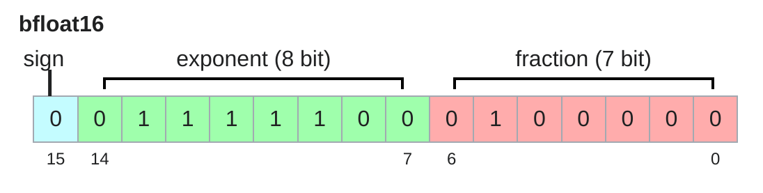
指数位和float32相同也就是说可以表示更接近于0的数了，精度有所下降，但是可以表示更小的数了，不至于让1.001变成1.000

也可以直接转成float32用于混合精度训练

fp8

nvidia提的

浮点数总结

总之不用FP32你会得到一个单词：instability不稳定的，因为会有下溢

tensor存储

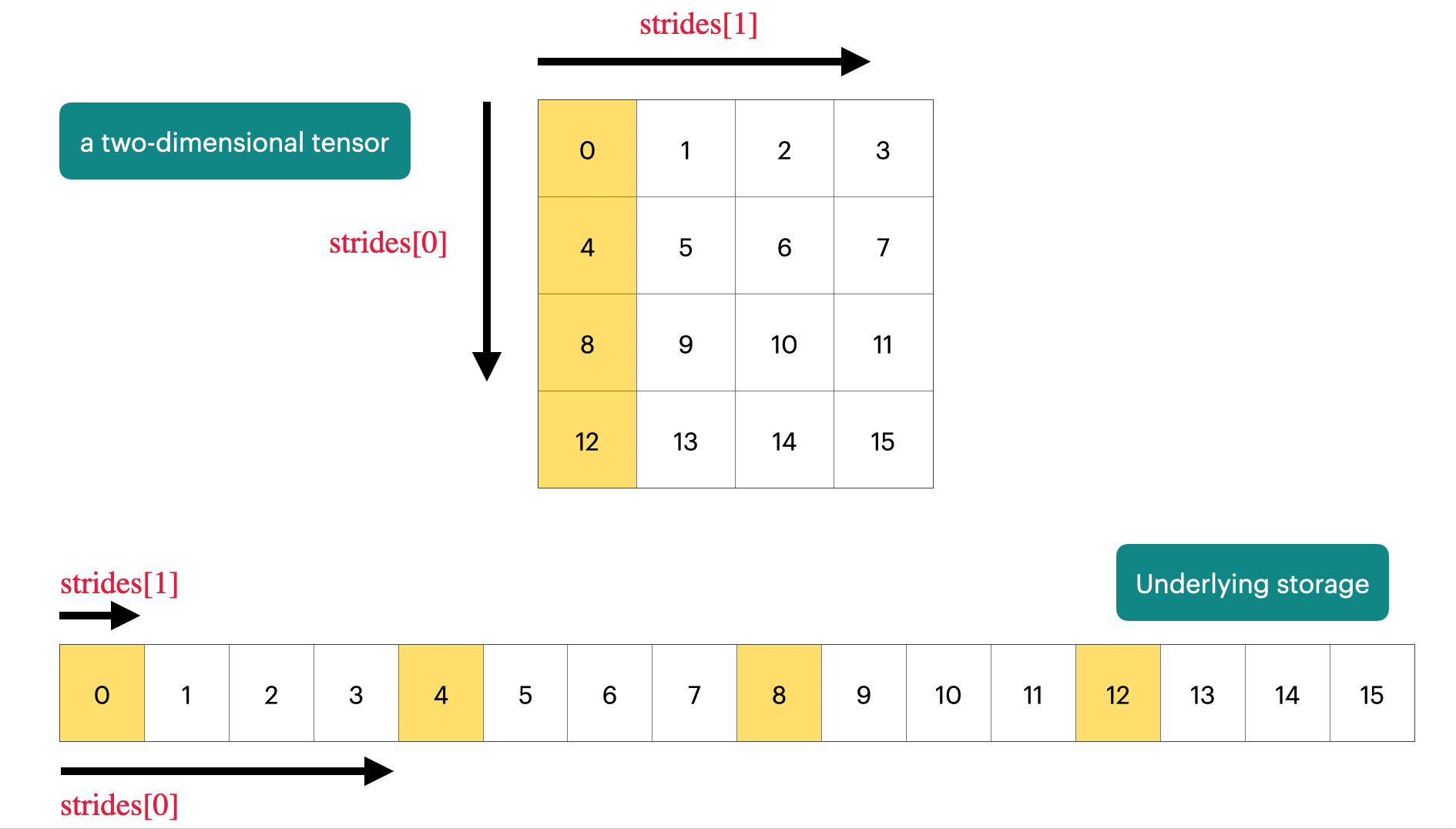
PyTorch 默认是 row-major (C-style) 连续存储，也就是最后一个维度在地址上是连续的。

然后很多切片操作和计算（原地计算）只是改变tensor的属性值没有改变内存地址

# Note that some views are non-contiguous entries, which means that further views aren't possible.
    x = torch.tensor([[1., 2, 3], [4, 5, 6]])  # @inspect x
    y = x.transpose(1, 0)  # @inspect y
    assert not y.is_contiguous()
    try:
        y.view(2, 3)
        assert False
    except RuntimeError as e:
        assert "view size is not compatible with input tensor's size and stride" in str(e)

这里是转置矩阵后内存还是按照顺序存的，访问顺序变了

y[0,0] -> 1
y[0,1] -> 4   (跳 3 个元素)
y[1,0] -> 2   (跳 1 个元素)
y[1,1] -> 5
...

可以用y.reshape(2, 3)或者 y = x.transpose(1, 0).contiguous().view(2, 3)

内存就变了不是一个地址了

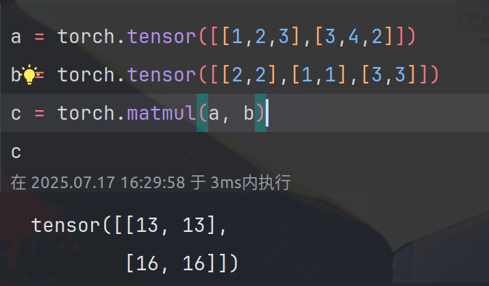
矩阵乘法

行与列进行点积后的结果

x @ w = torch.matmul(x, w)

einops

爱因斯坦标示

x = torch.ones(2, 2, 3)  # batch, sequence, hidden  @inspect x
y = torch.ones(2, 2, 3)  # batch, sequence, hidden  @inspect y
z = x @ y.transpose(-2, -1)  # batch, sequence, sequence  @inspect z

# jaxtyping
x: Float[torch.Tensor, "batch seq1 hidden"] = torch.ones(2, 3, 4)  # @inspect x
y: Float[torch.Tensor, "batch seq2 hidden"] = torch.ones(2, 3, 4)  # @inspect y

z = einsum(x, y, "batch seq1 hidden, batch seq2 hidden -> batch seq1 seq2") 

# Old way:
y = x.mean(dim=-1)  # @inspect y
# New (einops) way:
y = reduce(x, "... hidden -> ...", "sum")  # @inspect y

FLOP(floating-point operation)

• FLOPs: floating-point operations (measure of computation done)浮点运算次数（衡量计算量的指标）
• FLOP/s: floating-point operations per second (also written as FLOPS), which is used to measure the speed of hardware.每秒浮点运算次数（也写作FLOPS），用于衡量硬件的速度。

小写s代表总次数（统计、总和），大写S代表每秒的计算次数（衡量单位、指标）

if torch.cuda.is_available():
    B = 16384  # Number of points
    D = 32768  # Dimension
    K = 8192  # Number of outputs
else:
    B = 1024
    D = 256
    K = 64
device = torch.device('cuda' if torch.cuda.is_available() else 'cpu')
x = torch.ones(B, D, device=device)
w = torch.randn(D, K, device=device)
y = x @ w
# FLOPs = B × K × (2D−1)讲道理是这么算的，加法应该少一次，可能是D比较大把1忽略了？
actual_num_flops = 2 * B * D * K # 8796093022208

MFU

torch.cuda.get_device_properties(device)

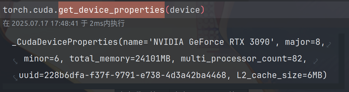
TF32 是 NVIDIA 为了加速训练在 Ampere 架构（如 A100）及以后推出的一种 权衡速度与精度的格式。尾数位只有10，后面位数全是0。

计算一下我3090实际的MFU

import timeit


def time_matmul(a: torch.Tensor, b: torch.Tensor) -> float:
    """Return the number of seconds required to perform `a @ b`."""
    # Wait until previous CUDA threads are done
    if torch.cuda.is_available():
        torch.cuda.synchronize()

    def run():
        # Perform the operation
        a @ b
        # Wait until CUDA threads are done
        if torch.cuda.is_available():
            torch.cuda.synchronize()

    # Time the operation `num_trials` times
    num_trials = 5
    total_time = timeit.timeit(run, number=num_trials)
    return total_time / num_trials


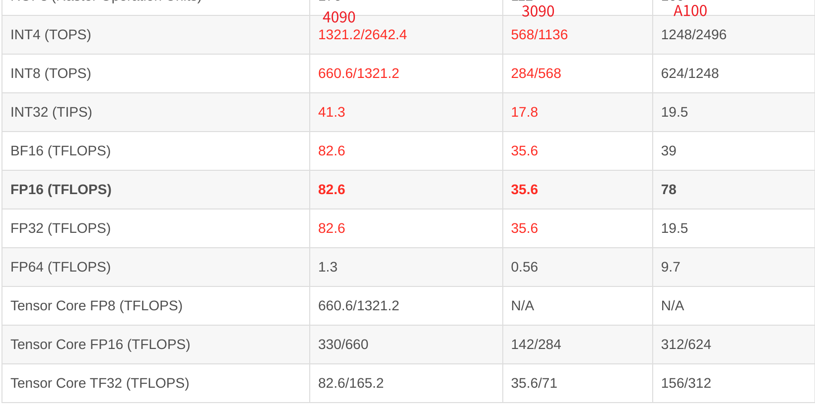
# 3090理论每秒FP32 FLOPS 35.6*e12
promised_flop_per_sec = 35.6e12
# 实际每秒
if torch.cuda.is_available():
    B = 16384  # Number of points
    D = 32768  # Dimension
    K = 8192  # Number of outputs
else:
    B = 1024
    D = 256
    K = 64
device = torch.device('cuda' if torch.cuda.is_available() else 'cpu')
x = torch.ones(B, D, device=device)
w = torch.randn(D, K, device=device)
y = x @ w
actual_num_flops = 2 * B * D * K
print("实际FLOPs：", actual_num_flops)
# 转成bfloat16
# x = x.to(torch.bfloat16)
# w = w.to(torch.bfloat16)
actual_time = time_matmul(x, w)
print("实际时间：", actual_time)
actual_flop_per_sec = actual_num_flops / actual_time
print("实际FLOPS：", actual_flop_per_sec)
mfu = actual_flop_per_sec / promised_flop_per_sec
print("MFU：", mfu)

这是默认的情况下：

• 实际FLOPs： 8796093022208
• 实际时间： 0.3723490708041936
• 实际FLOPS： 23623244186457.45
• MFU： 0.6635742749004901

BF16格式下：

• 实际FLOPs： 8796093022208
• 实际时间： 0.12506474698893727
• 实际FLOPS： 70332313733350.195
• MFU： 1.9756267902626459

这图片BF16的数据不对劲吧，MFU都1.97了，裂开

代码本地运行速度很明显BF16比FP32运行快多了

Gradient(backward)

# Forward pass: compute loss
x = torch.tensor([1., 2, 3])
w = torch.tensor([1., 1, 1], requires_grad=True)
y = x @ w
loss = 0.5 * (y - 5).pow(2)

# Backward pass: compute gradients
loss.backward()
print(w.grad) # tensor([1., 2., 3.])

∂loss/∂w = ∂loss/∂pred_y * ∂pred_y/∂w
∂loss/∂pred_y = (pred_y - 5) = 6 - 5 = 1
∂pred_y/∂w = x = [1, 2, 3]
因此：∂loss/∂w = 1 * [1, 2, 3] = [1, 2, 3]

计算梯度时的FLOPs

这里比较难理解啊

先贴一下原讲义（可以后面点开看）：

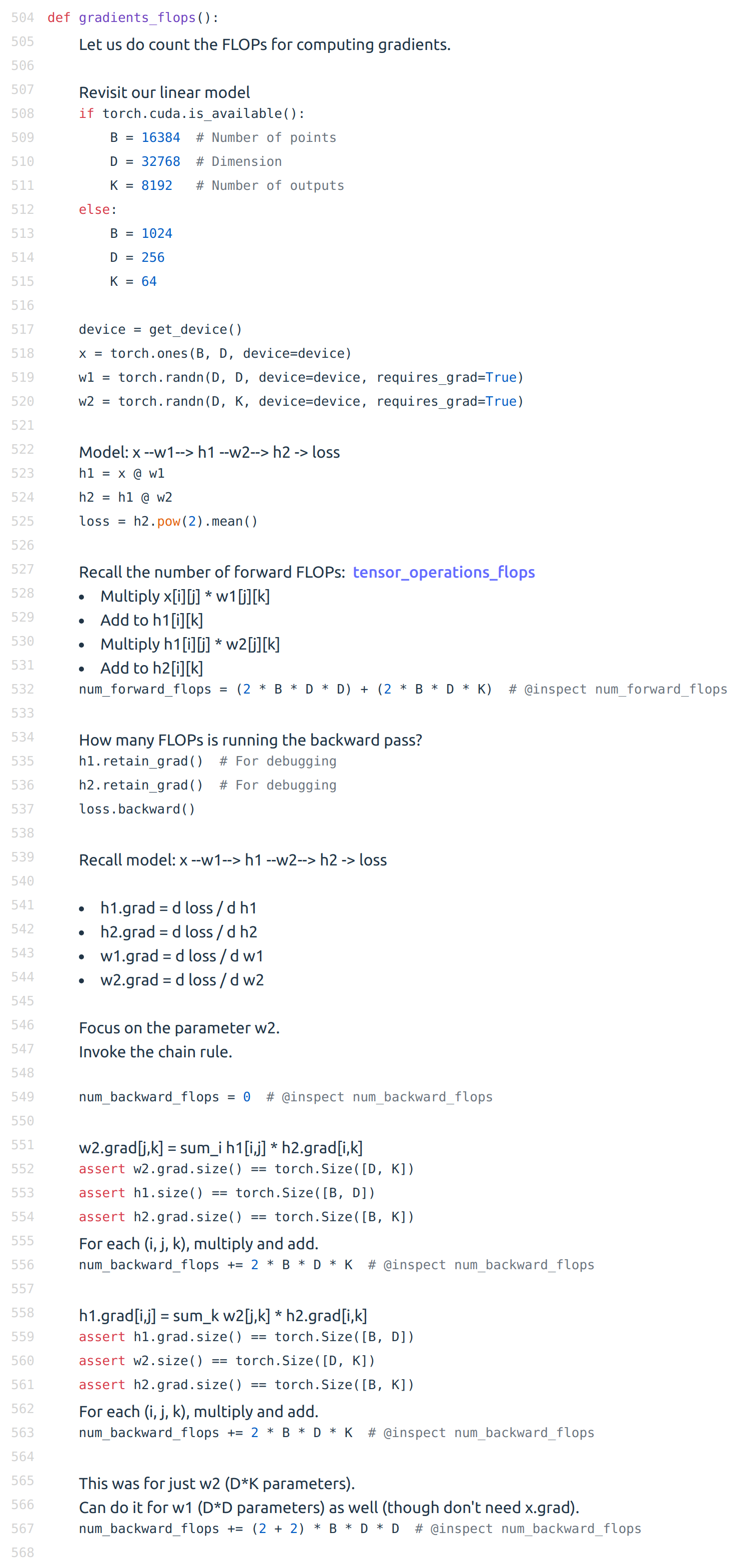
一开始的前向传播计算好理解点

从这开始How many FLOPs is running the backward pass?计算反向传播的FLOPs

这里写代码跑一遍

import torch

if torch.cuda.is_available():
    B = 6192  # Number of points
    D = 10240  # Dimension
    K = 4096  # Number of outputs
else:
    B = 1024
    D = 256
    K = 64

device = torch.device('cuda' if torch.cuda.is_available() else 'cpu')
x = torch.ones(B, D, device=device)
w1 = torch.randn(D, D, device=device, requires_grad=True)
w2 = torch.randn(D, K, device=device, requires_grad=True)

# 矩阵乘法 矩阵1：M*N 矩阵2: N*Q 算一个元素值乘法次数要 N次，加法要 N-1 次
# 总次数为 M * Q * (N + N -1) = M * Q * (2N - 1) 
# 1可以忽略不计 所以是 2 * M * Q * N

h1 = x @ w1  # Size: B D * D D -> B D FLOPs: 2 * B * D * D
h2 = h1 @ w2  # Size: B D * D K -> B K FLOPs: 2 * B * D * K
loss = h2.pow(2).mean()  # MSE 均方误差

num_forward_flops = (2 * B * D * D) + (2 * B * D * K)
print("Forward FLOPs:", num_forward_flops)

h1.retain_grad()  # For debugging
h2.retain_grad()  # For debugging
loss.backward()

# h1.grad = d loss / d h1
# h2.grad = d loss / d h2
# w1.grad = d loss / d w1

num_backward_flops = 0

# 计算w2的梯度：
# w2.grad = d loss / d w2 = d loss / d h2 * d h2 / d w2 = h2.grad * h1
# h2 第 i 行第 k 列的元素，由 h1 的第 i 行和 w2 的第 k 列相乘得到
# 所以：h2[i,k] = sum_j h1[i,j] * w2[j,k]
# 然后对w2求导：
# ∂h2[i,k]/∂w2[j,k] = h1[i,j]
# 下面做代换
# ∂loss/∂h2[i,k] = h2.grad[i,k]
# ∂loss/∂w2[j,k] = sum_i ∂loss/∂h2[i,k] * ∂h2[i,k]/∂w2[j,k]
# 得到：
# w2.grad[j,k] = ∂loss/∂w2[j,k] = sum_i h1[i,j] * h2.grad[i,k]

# 导数SIZE和本身是一样
assert w2.grad.size() == torch.Size([D, K])
# w2.grad[j,k] = sum_i h1[i,j] * h2.grad[i,k]
assert h1.size() == torch.Size([B, D])
assert h2.grad.size() == torch.Size([B, K])
# For each (i, j, k), multiply and add.
# 计算一次反向传播
num_backward_flops += 2 * B * D * K
print(num_backward_flops)

# h1.grad[i,j] = sum_k w2[j,k] * h2.grad[i,k]
assert h1.grad.size() == torch.Size([B, D])
assert w2.size() == torch.Size([D, K])
assert h2.grad.size() == torch.Size([B, K])
# For each (i, j, k), multiply and add.
num_backward_flops += 2 * B * D * K
print(num_backward_flops)
# This was for just w2 (D*K parameters).
# Can do it for w1 (D*D parameters) as well (though don't need x.grad).
num_backward_flops += (2 + 2) * B * D * D
print(num_backward_flops)

就是说反向传播计算梯度：要4 * B * D * K（自己算2 * B * D * K，传播给下面2 * B * D * K）加上前向就是 6 * B * D * K的FLOPs

A nice graphical visualization:

[article]

Putting it togther:

Forward pass: 2 (# data points) (# parameters) FLOPs

Backward pass: 4 (# data points) (# parameters) FLOPs

Total: 6 (# data points) (# parameters) FLOPs

这里Callback开头的（为什么是6）

Model

模型参数

import torch
from torch import nn
input_dim = 16384
output_dim = 32
w = nn.Parameter(torch.randn(input_dim, output_dim))
assert isinstance(w, torch.Tensor)  # Behaves like a tensor
assert type(w.data) == torch.Tensor  # Access the underlying tensor

x = nn.Parameter(torch.randn(input_dim))
output = x @ w 
assert output.size() == torch.Size([output_dim])
# output值：输出值在~sqrt(16384) ≈ ±128范围 标准正态分布
tensor([ 164.4998, -175.6749,  -56.8557, -105.4998, -236.2094,  -31.9990,
        -162.7417,  118.6591,  -34.7936,  153.1620, -179.9156,   54.2254,
         165.4161, -266.0403,  -47.7279,   33.3281,   93.2577,   24.5926,
         -97.0982, -135.6569, -140.1329,  -53.7529,   -8.4854,  -98.3632,
         323.0457,  -55.9706,  -55.4370,   61.9023,  103.4207,  179.0014,
         101.8132,  -22.8997], grad_fn=<SqueezeBackward4>)

强调的是模型参数的初始化：

output值过大导致后面的梯度爆炸各种不稳定，所以就是缩放初始值

w = nn.Parameter(torch.randn(input_dim, output_dim) / np.sqrt(input_dim))

再进一步截断正态分布

# To be extra safe, we truncate the normal distribution to [-3, 3] to avoid any chance of outliers.
w = nn.Parameter(nn.init.trunc_normal_(torch.empty(input_dim, output_dim), std=1 / np.sqrt(input_dim), a=-3, b=3))

截断正态分布（Truncated Normal Distribution） ，目的是为了避免初始化中出现极端值（outliers），从而让训练更稳定。

提高神经网络训练的稳定性和收敛速度

自定义模型

import numpy as np
import torch
from torch import nn


def get_num_parameters(model: nn.Module) -> int:
    return sum(param.numel() for param in model.parameters())


class Cruncher(nn.Module):
    def __init__(self, dim: int, num_layers: int):
        super().__init__()
        self.layers = nn.ModuleList([
            Linear(dim, dim)
            for i in range(num_layers)
        ])
        self.final = Linear(dim, 1)

    def forward(self, x: torch.Tensor) -> torch.Tensor:
        # Apply linear layers
        B, D = x.size()
        for layer in self.layers:
            x = layer(x)
        # Apply final head
        x = self.final(x)
        assert x.size() == torch.Size([B, 1])
        # Remove the last dimension
        x = x.squeeze(-1)
        assert x.size() == torch.Size([B])
        return x


class Linear(nn.Module):
    """Simple linear layer."""

    def __init__(self, input_dim: int, output_dim: int):
        super().__init__()
        self.weight = nn.Parameter(torch.randn(input_dim, output_dim) / np.sqrt(input_dim))

    def forward(self, x: torch.Tensor) -> torch.Tensor:
        return x @ self.weight


D = 64  # Dimension
num_layers = 2
model = Cruncher(dim=D, num_layers=num_layers)

param_sizes = [
    (name, param.numel())
    for name, param in model.state_dict().items()
]
print(param_sizes)
assert param_sizes == [
    ("layers.0.weight", D * D),
    ("layers.1.weight", D * D),
    ("final.weight", D),
]
num_parameters = get_num_parameters(model)
print(num_parameters)
assert num_parameters == (D * D) + (D * D) + D

device = torch.device('cuda' if torch.cuda.is_available() else 'cpu')
model = model.to(device)

B = 8  # Batch size
x = torch.randn(B, D, device=device)
y = model(x)
print(y)
assert y.size() == torch.Size([B])

输出：

[('layers.0.weight', 4096), ('layers.1.weight', 4096), ('final.weight', 64)]
8256
tensor([ 0.4874,  0.7666,  0.7967, -0.1383,  2.1578, -0.9054,  0.5778, -1.0364],
       device='cuda:0', grad_fn=<SqueezeBackward1>)

随机

同步随机种子

 # Torch
seed = 0
torch.manual_seed(seed)
# NumPy
import numpy as np
np.random.seed(seed)
# Python
import random
random.seed(seed)

数据加载

懒加载

orig_data = np.array([1, 2, 3, 4, 5, 6, 7, 8, 9, 10], dtype=np.int32)
orig_data.tofile("data.npy")
data = np.memmap("data.npy", dtype=np.int32)
assert np.array_equal(data, orig_data)

Pinned memory

固定内存

if torch.cuda.is_available():
    x = x.pin_memory()

This allows us to copy x from CPU into GPU asynchronously.

• x = x.to(device, non_blocking=True)

This allows us to do two things in parallel (not done here):

• Fetch the next batch of data into CPU
• Process x on the GPU

优化器 - optimizer

Let’s define the AdaGrad optimize

• momentum = SGD + exponential averaging of grad
• AdaGrad = SGD + averaging by grad^2
• RMSProp = AdaGrad + exponentially averaging of grad^2
• Adam = RMSProp + momentum

AdaGrad: https://www.jmlr.org/papers/volume12/duchi11a/duchi11a.pdf

from typing import Iterable


class AdaGrad(torch.optim.Optimizer):
    def __init__(self, params: Iterable[nn.Parameter], lr: float = 0.01):
        super(AdaGrad, self).__init__(params, dict(lr=lr))

    def step(self):
        for group in self.param_groups:
            lr = group["lr"]
            for p in group["params"]:
                # Optimizer state
                state = self.state[p]
                grad = p.grad.data
                # Get squared gradients g2 = sum_{i<t} g_i^2
                g2 = state.get("g2", torch.zeros_like(grad))
                # Update optimizer state
                g2 += torch.square(grad)
                state["g2"] = g2
                # Update parameters
                p.data -= lr * grad / torch.sqrt(g2 + 1e-5)

B = 2
D = 4
num_layers = 2
model = Cruncher(dim=D, num_layers=num_layers)
optimizer = AdaGrad(model.parameters(), lr=0.01)
model.to(device)
model.state_dict()

# 参数
OrderedDict([('layers.0.weight',
              tensor([[ 0.0738,  0.0796,  0.7888,  0.2291],
                      [-0.5016, -0.6035, -0.7239, -0.5630],
                      [ 0.6271,  0.5637, -0.5113, -0.5344],
                      [ 0.4712, -0.3981,  0.1651,  0.3281]], device='cuda:0')),
             ('layers.1.weight',
              tensor([[ 0.0183, -0.0411,  0.4005, -0.6554],
                      [-0.7396, -0.9855,  0.0469, -0.6268],
                      [-0.0726, -0.3529,  0.0033,  0.3119],
                      [-0.1595,  0.3192,  0.0668, -1.0775]], device='cuda:0')),
             ('final.weight',
              tensor([[ 0.7161],
                      [-0.6522],
                      [-0.2452],
                      [ 0.0712]], device='cuda:0'))])

import torch.nn.functional as F

x = torch.randn(B, D, device=device)
y = torch.tensor([4., 5.], device=device)
pred_y = model(x)
loss = F.mse_loss(input=pred_y, target=y)
loss.backward()
optimizer.step()
model.state_dict()

# 参数
OrderedDict([('layers.0.weight',
              tensor([[ 0.0638,  0.0896,  0.7988,  0.2191],
                      [-0.5116, -0.5937, -0.7139, -0.5730],
                      [ 0.6171,  0.5737, -0.5013, -0.5444],
                      [ 0.4812, -0.4081,  0.1551,  0.3381]], device='cuda:0')),
             ('layers.1.weight',
              tensor([[ 0.0083, -0.0311,  0.4105, -0.6653],
                      [-0.7296, -0.9955,  0.0369, -0.6168],
                      [-0.0826, -0.3429,  0.0132,  0.3026],
                      [-0.1695,  0.3292,  0.0768, -1.0875]], device='cuda:0')),
             ('final.weight',
              tensor([[ 0.7061],
                      [-0.6622],
                      [-0.2552],
                      [ 0.0812]], device='cuda:0'))])

# Free up the memory (optional)
optimizer.zero_grad(set_to_none=True)

内存 - Memory

# Parameters
num_parameters = (D * D * num_layers) + D
print(num_parameters)
# Activations
num_activations = B * D * num_layers
print(num_activations)
# Gradients
num_gradients = num_parameters
print(num_gradients)
# Optimizer states
num_optimizer_states = num_parameters
print(num_optimizer_states)
# Putting it all together, assuming float32
total_memory = 4 * (num_parameters + num_activations + num_gradients + num_optimizer_states)
print(total_memory)
# FLOPs
flops = 6 * B * num_parameters
print(flops)

# results
36
16
36
36
496
432

训练循环 - Train Loop

class SGD(torch.optim.Optimizer):
    def __init__(self, params: Iterable[nn.Parameter], lr: float = 0.01):
        super(SGD, self).__init__(params, dict(lr=lr))

    def step(self):
        for group in self.param_groups:
            lr = group["lr"]
            for p in group["params"]:
                grad = p.grad.data
                p.data -= lr * grad


def get_device():
    return torch.device('cuda' if torch.cuda.is_available() else 'cpu')


def train(name: str, get_batch,
          D: int, num_layers: int,
          B: int, num_train_steps: int, lr: float):
    model = Cruncher(dim=D, num_layers=0).to(get_device())
    optimizer = SGD(model.parameters(), lr=0.01)
    for t in range(num_train_steps):
        # Get data
        x, y = get_batch(B=B)
        # Forward (compute loss)
        pred_y = model(x)
        loss = F.mse_loss(pred_y, y)
        # Backward (compute gradients)
        loss.backward()
        # Update parameters
        optimizer.step()
        optimizer.zero_grad(set_to_none=True)
        
D = 16
true_w = torch.arange(D, dtype=torch.float32, device=get_device())


def get_batch(B: int) -> tuple[torch.Tensor, torch.Tensor]:
    x = torch.randn(B, D).to(get_device())
    true_y = x @ true_w
    return (x, true_y)


print(get_batch(2))
train("simple", get_batch, D=D, num_layers=0, B=4, num_train_steps=10, lr=0.01)
train("simple", get_batch, D=D, num_layers=0, B=4, num_train_steps=10, lr=0.1)

ckpt - checkpoint

Training language models take a long time and certainly will certainly crash.

certainly will：当然会，势必

model = Cruncher(dim=64, num_layers=3).to(get_device())
optimizer = AdaGrad(model.parameters(), lr=0.01)
checkpoint = {
    "model": model.state_dict(),
    "optimizer": optimizer.state_dict(),
}
# Save the checkpoint:
torch.save(checkpoint, "model_checkpoint.pt")
# Load the checkpoint:
loaded_checkpoint = torch.load("model_checkpoint.pt")

mixed_precision_training

混合精度训练

A concrete plan:

• Use {bfloat16, fp8} for the forward pass (activations).
• Use float32 for the rest (parameters, gradients).

tradeoffs：权衡取舍